Standard Error of Measurement (SEM)
The SEM allows us to estimate the potential difference between a student’s obtained score and their true score. In Chapter 10, “Establishing Evidence of Reliability and Validity,” the implications of SEM on test score interpretation are discussed.
Understanding the importance of SEM is crucial because assuming that an obtained score on a test represents the student’s true score can lead to misinterpretation of test results (Reynolds et al., 2008). For our sample in Table 11.1, the SEM is 3.8, indicating that the true score for an observed raw score of 72 would fall within the range of 68.2 to 75.8. This range is referred to as the confidence band.
If a passing score on a test is set at 75, it might be tempting to add 4 points to all scores on the test when the SEM is 4. However, it is not advisable to scale grades for individual tests. Instead, it is better to wait for the final grade. Scaling individual test scores can disrupt the predetermined weighting of course components. The recommended practice is to wait until the end of the course, assess various factors like means, medians, reliability coefficients, SEMs for all exams, and the final score spread, and then consider adding points to the final grade assignment (refer to Chapter 13, “Assigning Grades” for more on grading).
The key lesson from the Standard Error of Measurement (SEM) is that classroom test scores are not absolute representations of students’ true scores. Measurement error exists in all scores, so it is essential to consider the margin of error in a test and be flexible when translating raw scores into test scores and course grades. If your test development software does not provide the SEM, you can calculate it using the formula in Exhibit 10.5.
Score Distribution
A test score distribution complements test data analysis by providing an overview of how the entire class performed on the test. Distributions help visualize test results and make scores easier to interpret. Typically reported in a frequency table or graphic format, score distributions provide valuable insights.
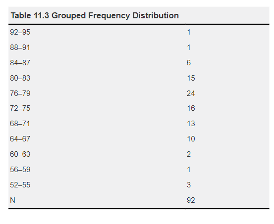
Table 11.3 presents a grouped frequency distribution for the sample data in Table 11.1, grouping raw scores into four-point intervals. This distribution allows us to see, for instance, that six students scored between 84 and 87. It provides a visual representation of the range of raw scores on the test, aiding the interpretation of data such as the mean and median and identifying score clustering.